Temporal Difference in Reinforcement Learning

Abstract

The purpose of this paper is to revisit the article, “Learning to Predict by the Methods of Temporal Differences” (1988) by Richard Sutton and replicate some of the experiments therein. In his article, Sutton introduced and formalized the theory of temporal-difference (TD) methods, which are a subset of general prediction methods. Sutton goes on to describe the advantages of TD methods over supervised learning methods when predicting dynamical systems, systems which have states evolving over time. Sutton provided a simple dynamical system, a random walk, and produced experiments showing TD methods having improved learning with lower error rates than a comparable supervised learning algorithm.

Introduction and Background

This paper contains an overview of temporal-difference (TD) methods and to reengineer experiments on TD methods from an academic paper by Richard Sutton. TD methods provide an avenue for deriving the best policy for navigating multi-step systems and systems with delayed results. A policy, in this case, provides a recommended next best action to an agent given any state within a system. Examples of such systems include games (ex: Chess), predicting the weather, forecasting stock market volatility or other pattern-recognition scenarios.

There are other types of algorithms to “learn” about a given system. For example, Dynamic Programming (DP) methods involve simulating many episodes within a system where the value of a given state is determined by the values of all potential states one step beyond the state. In contrast, Monte Carlo (MC) methods involve deriving the value of a given state based only on the terminal states found in episodes containing that state. Where DPmethods can be thought of as 1-step lookahead learning methods and MC methods are last-step learning methods, TD methods handle both extremes while also taking into account “middle-ground” scenarios. In fact, TD methodology unifies the MC and DP methodology while under a single algorithm as well as middle-ground values for faster, more efficient learning. This algorithm is known as TD($\lambda$) where $0 \leq \lambda \leq 1$ with TD(0) and TD(1) equivalent to DP and MC methods respectively.

Like any learning algorithm, TD methods “learn” by updating its weights:

$\Delta w_t = \alpha(z - P_t)\triangledown_w P_t$

“Weights” can also be considered the perceived value of a given value state, $z$ as the reward of the terminal state, $\alpha$ is a positive learning rate, $P_t$ as the vector of state values, and $\triangledown_w P_t$ is the partial derivative of $P_t$ with respect to $w$. This effectively isolates the one-to-one relationship of weight/value to a given state as the partial derivative converts all other values to 0. The TD($\lambda$) algorithm’s weight changing $\delta w_t$ formula is an evolution of that formula above because it can update its “learning” through incremental steps:

$\Delta w_t = \alpha(P_{t+1} - P_t) \sum_{n=1}^T \lambda^{T-n} \triangledown_wP_k$

Where $t$ is time step within $1 \leq t \leq T$ and $T$ is the total number of steps in a given episode of a system. While TD(0) (Monte Carlo) is a 1 step process process and TD(1) (Dynamic Programming) is a last step process, the equation above takes into account every step, n-step, from 1 to $T$ where the impact of a proceeding state on the value function of the current state is degraded by the exponential decay $\lambda^{T-n}$ so that the closer states have a stronger impact. However, rather than iterating through all of the n-steps for each state sequentially, we can actually shorten the computation by vectorizing the equation. We can do this by providing an eligibility trace, vector $e$, with all values in the vector initially set to zero. When the algorithm iterates through an episode,$S_{t-1} \rightarrow S_t$, then $e_{t-1} = e_{t-1} + 1$ such that only the states visited in the sequence so far are updated during the weight change.

$\Delta w_t = \alpha(P_{t+1} - P_t) \lambda e_{t+1}$

With the equation above, we can iteratively search through and learn from a dynamical system. In Sutton’s paper, he provided a random walk scenario as a simple dynamical system that we can use to observe TD(\lambda) performance. The random walk system from Sutton’s paper consists of seven linearly connected states (A, B, C, D, E, F, G) where A and G are terminal states and each episode has the agent start on state D. Each state has a 50% chance of transitioning to the state to its left and a 50% to its right with every state having a reward value of zero except for the G state which has a reward of one. A given episode in this system records all the transitions the agent makes until the agent hits one of the terminal states. The learning algorithm is thus trying to approximate what the expected value of each non-terminal state of the system which are $\frac{1}{6},\frac{1}{3},\frac{1}{2}, \frac{2}{3},$ and $\frac{5}{6}$ for states B, C, D, E, and F.

For the experiments in Sutton’s paper regarding the random walk system, we replicate the steps he used in creating training data by generating 100 unique training sets with each set containing 10 randomly generated random walk episodes for a total of 1000 episodes. For each experiment, we compare the expected values the learning algorithm generates from each training set with the true values stated above, derive the root mean squared error (RMSE) for each set, and then mean average the errors from all 100 sets as the output to compare how different values of $\lambda$ perform for TD($\lambda$).

Experiment 1

The first experiment in Sutton’s paper regarding random walks was comparing how TD($\lambda$) performed against a base linear supervised learning module, which TD(1) replicates, under repeated training over a small amount of training data. Sutton wanted to compare the base learning of TD($\lambda$) compared to supervised learning algorithms so he even modified the TD($\lambda$) learning algorithm so that the weights would not update incrementally but update at the end of a training set so to provide an apples to apples comparison with supervised learning algorithms. The compared supervised learning algorithm in this instance is represented using TD(1). The different models of TD($\lambda$) are repeatedly shown the same 10 sequences of a training set, updating at their weights at the end of the training set, and do not stop until the max value within the $\Delta w_t$ vector is below a certain threshold value.

Experiment 1 Results

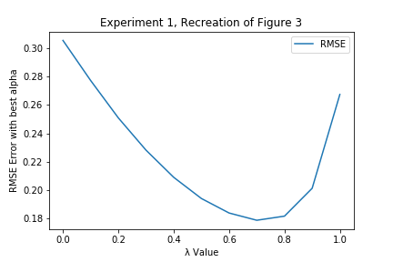
The results derived from trying to reengineer Sutton’s work match up quite well to the original material with any data point being at most +/- 0.1 from the values Sutton derived. I attribute these differences to possible floating point arithmetic errors, and the potential different number significant digits used in optimizing $\alpha$. These results show how, for TD($\lambda$) values less than 1 perform better than TD(1). In this case, we can see the best $\lambda$ is either 0 or 0.1. This outperformance over TD(1) is attributed to the fact that TD(1) minimizes error strictly to the training set while smaller values for $\lambda$, which considers other states besides the end state, attempt to minimize the error for future experiences. This consideration for intermediate states enables the algorithms to take into account how far away a given state is from its terminal reward state and adjust accordingly in a way that a simple one-to-one mapping of a baseline supervised learning algorithm cannot.

Experiment 1 Replication Shortfalls and Assumptions

There were significant hurdles replicating the first random walk experiment in Sutton’s paper as Sutton does not go into detail about how he altered the TD($\lambda$) algorithm to not update weights until the end of a training set. Simply summing the ten $\Delta w_t$’s meant that the explored $\alpha$ ranges would have to be several magnitude smaller smaller than otherwise would be explored in order for $\Delta w_t$ to converge. This meant that certain $\lambda$ values would only converge at $\alpha$ values small enough to be impacted by Python floating point errors. In order to combat this, I would divide every $\Delta w_t$ by the number of sequences (10) in order to have larger learning rates that would still converge. It also meant that the $\alpha$ used in Experiment 1 would not be the same as those used in Experiment 2. Since Sutton did not provide the $\alpha$ values used in Experiment 1 nor a threshold stopping condition $D$ for training where $|\Delta w_{t+1} - \Delta w_t| > D$, I settled for a stopping threshold of 0.0001.

Experiment 2

While Sutton’s first experiment observed the advantage of TD($\lambda$) under repeated training scenarios, the second experiment was meant to observe TD($\lambda$)’s learning speed with only a nominal amount of data. Rather than being repeatedly shown the same training set like in the first experiment, the different models of TD($\lambda$) were shown a training set exactly once. Also, unlike in the first experiment when models updated their weights at the end of a training set, the second experiment had models update their weights at the end of every sequence. The RMSE for each training set were then collected and averaged out to see the average performance of initial learning for different values of $\lambda$. Since a training set was only observed once, the projected expected values would not have enough time to converge. In order to minimize bias in the results, each model’s value function vector was initially set to 0.5.

Experiment 2 Results

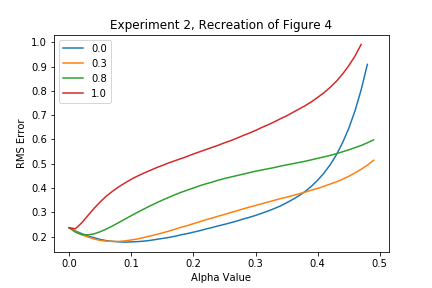
For this experiment, Sutton first compared the combinations of different $\lambda$ and $\alpha$ values. Recreating the experiment yielded results very similar to those found in Sutton’s paper. The relative performance of the 4 different $\lambda$ values is consistent between papers with TD(1), the supervised learning algorithm, immediately performing the worst for any positive $\alpha$ and $\lambda =0$ performing well for small $\alpha$ values before exponentially increasing its RMSE around $\alpha =0.35$. In comparison, the intermediate $\lambda$ values 0.3 and 0.8 find their global minima in positive values and both have much flatter slopes than TD(0) or TD(1) suggesting less sensitivity to hyper-parameter tuning like learning rate.

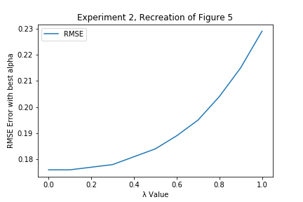
By graphing the RMSE for different values of $\lambda$ with their optimized $\alpha$ values, we can observe once again how intermediate values for $\lambda$ perform better than either of their extremes at TD(0) and TD(1). The recreated results for Experiment 2 have slightly different results than what Sutton produced in that all the values seemed to have a 0.03-0.06 increase in their RMSE values in the recreated results. At the same time though, the observations from the original paper still hold where the optimal value for TD($\lambda$) is 0.3. While the first experiment did not really show a valuable improvement for TD($\lambda$) compared to TD(0), we can see in these results that TD() learns faster than TD(0) because it can simultaneously update all states whereas TD(0)’s forward propagation can only update one state at a time for every step in the sequence. While TD(0) can avoid this issue through backpropagation, doing so eliminates its ability to do incremental learning.

Experiment 2 Replication Shortfalls and Assumptions

Trying to recreate Sutton’s results for Experiment 2 led to new results that seemed to have a near constant-value positive difference from the original values. Since the difference is relatively constant and the TD($\lambda$) improvements are observable in both results, the differences can be considered trivial. The difference suggest some sort of gamma constant applied to the $\Delta w_t$ which wasn’t previously mentioned or slightly different state space searches for optimal values. Neither of these possible shortfalls detract from the overall findings.

Conclusion

Through these experiments of algorithm performance on a random walk system, we can see the the improved learning of a TD($\lambda$) algorithm with a value $0 < \lambda < 1$ compared to Monte Carlo and Dynamic Programming methods in dynamical systems. TD($\lambda$) achieves both a lower average error with a smaller amount of data (Experiment 1), which beats TD(1), and a faster learning rate (Experiment 2), which is better than both TD(0) and TD(1). I also observed that, while I could not 100% replicate Sutton’s results, the recreated results were close and maintained the same data relationships and findings as what was observed in Sutton’s work thus verifying the validity of the TD methodology.