Bayesian Approach to Portfolio Allocation

1. Introduction

One of the main services of investment management is to construct portfolios of stocks and bonds (securities) for clients that provides the best risk-adjusted returns. A significant amount of research has gone into portfolio construction including the invention of mean-variance optimization. Harry Markowitz introduced mean-variance optimization in 1952 and received a Nobel prize in Economics for this research. Mean-variance optimization, also known as Modern Portfolio Theory (MPT), has been the cornerstone of portfolio construction since, but it is not without issues.

After a portfolio manager (PM) decides which securities to invest in, the PM must decide what percentage of the portfolio to invest in each security. Mean-variance optimization (MVO) is a method to discover this optimal weighting. In order to accomplish this, MVO computes the volatility (standard deviation) of the portfolio which requires assembling a covariance matrix ($\Sigma$) of the relationships of all the different security returns. Once this is complete, MVO searches through an assortment of weights in order to maximize risk-adjusted returns known as the Sharpe Ratio:

$\text{Sharpe Ratio} = \frac{R_p - R_f}{\sigma_p}, \quad R_p = \text{expected portfolio return }$

$R_f = \text{risk free rate}, \quad \sigma_p = \text{portfolio volatility}, \quad w = \text{vector of weights}$

$\sigma_p = \sqrt{\sigma_p^2}, \quad \sigma_p^2 = w^T\Sigma w$

$MVO = max(\frac{R_p - R_f}{\sigma_p})$

3 Asset Portfolio Example:

$$\sigma_p^2 = \begin{bmatrix} 0.3 & 0.4 & 0.3 \end{bmatrix} \bullet \left( \begin{bmatrix} 0.1 & 0.2 & 0.3 \\ 0.4 & 0.5 & 0.4 \\ 0.3 & 0.2 & 0.1 \end{bmatrix} \bullet \begin{bmatrix} 0.3 \\ 0.4 \\ 0.3 \end{bmatrix} \right)$$ $$\sigma_p^2 = \begin{bmatrix} 0.3 & 0.4 & 0.3 \end{bmatrix} \bullet \begin{bmatrix} 0.2 \\ 0.44 \\ 0.2 \end{bmatrix}$$

$\sigma_p^2 = 0.296$

These covariance matrices are extremely fragile; they are time-dependent, too precise, and degrade in terms as the number of unique stocks and bonds in the portfolio increase (creating larger matrices). Because of this fragility, pure MVO is not used much in practice as PMs attempt to find better methods to create low volatility portfolios that are resilient against unknown future risks. This paper attempts to recreate a Bayesian modeling approach to portfolio optimization that was previously explored by Fischer Black and Robert Litterman in their Black-Litterman models.

2. Data Source

For this experiment, I chose to optimize the weights of a portfolio of four ETFs (exchange traded funds) from the investment management firm Vanguard:

• Total Bond Market (BND)
• Total International Bond (BNDX)
• Total International Stock (VXUS)
• Total Stock Market (VTI)

I chose these four ETFs because combined they represent a vast majority of the investment trading universe as each is a proxy for their respective markets. They are also the four underlying investment products Vanguard uses when creating portfolios for clients through their financial advisor, robo-advisor, and target date fund offerings. This portfolio construction strategy is not exclusive to Vanguard but representative of the robo-advisor and retail investor portfolio construction offerings provided by the entire investment management industry. The combined assets of those 4 funds alone is $1.476 Trillion. Since this portfolio of “total” ETFs represents a significant chunk of most people’s investment and retirement account, any improvement in portfolio modeling here would be a huge boon for the average investor.

For this experiment, I am going to provide 3 years worth of data (April 1st 2016 - March 30th 2019) to optimize weights by Sharpe Ratios, and then test how those strategies play out from April 1st 2019 - March 30th 2020. This means the portfolios will be tested on their performance in the market recession caused by the Covid-19 pandemic which is a strong test on how risk resilient the portfolios are.

3. Creating the Models

One avenue of research is to replace the single covariance matrix of MVO by sampling returns and covariances through a Bayesian Markov Chain Monte Carlo (MCMC) approach. By sampling from a distribution of covariances, a Bayesian approach would potentially be more resilient to covariance outliers and present more genuine relationships among the different securities within a portfolio. I created two different models with the following parameters:

Model 1

Priors:

$\mu_i \sim N(0, \mu = 0.1), \quad \sigma_i \sim \text{HalfCauchy}(x_0=0, \gamma=5)$ $L \sim LKJ(\eta=5, \sigma_i), \quad \nu \sim Exp(0.1), \quad \Sigma = LL^T$

Posterior: $\mu \sim stt(\mu_i, \nu, \Sigma)$

Model 2

Priors:

$\mu_i \sim N(0, \mu = 0.1), \quad \sigma_i \sim \text{HalfCauchy}(x_0=0, \gamma=5)$ $L \sim LKJ(\eta=5, \sigma_i), \quad \Sigma = LL^T$

Posterior: $\mu \sim N(\mu_i, \Sigma)$

I used the a Student T distribution (ST) for predicting returns in the 1st model as ST has fatter tails than a normal distribution. Since stock returns have more extreme swings than a normal distribution accounts for, a Student T distribution may be more appropriate. As such, I will compare the Student T posterior to a Normal distribution

For the covariance matrix, I used a Lewandowski-Kurowick-Joe (LKJ) distribution which creates a prior on the correlation matrix. I then use a Cholesky Decomposition ($\Sigma = LL^T$) to convert the correlation matrix into a covariance matrix. This method is handling covariance matrix priors is computationally superior than creating covariance priors outright.

4. Results

Strategy	BND	BNDX	VTI	VXUS	In Sample Sharpe	Out Sample Sharpe
Classic MVO	0.00	86.13	13.87	0.00	1.748	0.462
Normal	3.76	82.28	13.94	0.01	1.748	0.478
StudentT	0.00	77.11	22.89	0.00	1.643	0.200

As the results show, the Normal Bayesian approximation from the returns yielded an identical in-sample Sharpe Ratio as the basic mean-variance optimization even though the they have slightly different portfolio compositions. Yet the Bayesian optimized portfolio actually performed better in terms of risk-adjusted returns in the out-sample. The Student-T distribution performed worse suggesting, at least in this instance, it is not as strong of a modeling agent. This would make sense since, while individual securities definitely do not have normal distributions of returns, a representation of an entire market, may exhibit more normal distribution qualities. We can see the close relationship of the classic MVO with the Bayesian Normal approximation performance in the chart below.

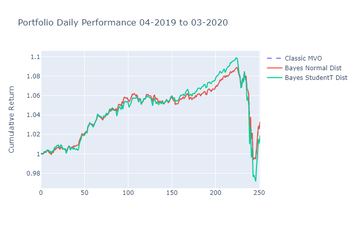
The Bayesian approximation maps extremely closely to the classic MVO path but, with the extra diversification, it is slightly less volatile and has handled the Covid-19 black-swan event slightly better.

5. Conclusion

In my analysis, I’ve shown how a Bayesian approximation can model a mean variance optimization. While in this specific instance, a Bayesian model was able to slightly beat the basic MVO approach, further research and more model tuning needs to occur before a definitive answer could be made on the effectiveness on the approach.

6. Errata

The code for this analysis was created with assistance and inspiration from the following sources:

• LKJ Cholesky Covariance Priors for Multivariate Normal Models¶
• Stochastic Volatility model
• Bayesian Portfolio Optimization